Introduction to R – Charts and Graphics

R includes several packages for visualizing data:

• graphics contains plotting functions for the “base” graphing systems, including plot, hist, boxplot and many others.
• lattice contains code for producing Trellis graphics, which are independent of the “base” graphics system; including functions like xyplot, bwplot, levelplot. It built on grid which implements a different graphing system independent of the “base” system.
• grDevices contains all code implementing the various graphics devices, including X11, PDF, PostScript, PNG, etc.

before making you chart, you need to think in the following:

• To what device will the chart be sent ? The default on windows is windows, on Mac OS X it is quartz, on Unix it is x11. You can find a list of devices available on your system in ?Devices
• Is The chart for viewing temporarily on the screen, or will it eventually end up in a paper ? Are you using it in a presentation ? charts included in a paper/presentation need to use a file device rather than a screen device.
• Is there a large amount of data going into the chart ? Or is it just a few points ?
• Do you need to be able to resize the chart ?
• What graphics system will you use: base or grid/lattice ?
• Base graphics are usually constructed with each aspect of the chart handled separately through a series of function calls; this is often conceptually simpler and allows plotting to mirror the thought process.
• Lattice/grid graphics are usually created in a single function call, so all of the graphics parameters have to be specified at once; specifying everything at once allows R to automatically calculate the necessary spacings and font sizes.

You can close the graphics device for your system with dev.off() or set it by dev.set() or turn all the graphics devices with graphics.off().

The base graphics system has many parameters that can set and tweaked for the whole session using par() function. Any of these parameters can be overridden as arguments to specific plotting functions. Some important parameters are:

• pch the plotting symbol (default is open circle). For more options run example(points)
• lty the line type (default is solid line). More information here
• lwd the line width, specified as an integer.
• col the plotting color, specified as a number, string, or hex code; the colors function gives you a vector of colors by name.
• las the orientation of the axis labels on the plot. More information here
• bg the background color
• mar the margin size
• oma the output margin size

you can get the default value of a parameter by par(“param_name”)

Plotting function

• plot make a scatterplot, or other type of plot depending on the class of the object being plotted.
• lines add lines to a plot, given a vector x values and a corresponding vector of y values (or a 2-column matrix); this function just connects the dots
• points add point to a plot
• text add text lebels to a plot using specified x, y coordinates
• title add annotations to x, y axis labels, title, subtitle, out margin
• mtext add arbitrary text to the margins (inner or outer) of the plot
• axis adding axis ticks/labels

now try to add some red points to it (this can be used make different types of points on the same scatterplot)

Now lets create a plot in a PDF file.

nothing will appear on the screen but a file names “testPlot.pdf” will be created in your working directory and contains the histogram. Notice that you have to call dev.off() to close the PDF device.

Copying plots

You can copy your plot to another device. This is useful because some plots require a lot of code and it can be a pain to type all that in again for a different device.

• dev.copy copy a plot from one device to another
• dev.copy2pdf copy a plot to a PDF file
• dev.list show a list of open graphics devices
• dev.next switch control to the next graphics device on the device list
• dev.set set control to a specific graphics device
• dev.off close the current graphics device

 

Plotting with lattice graphics

Major lattice functions

• xyplot the main function for creating scatterplots
• bwplot for box-and-whiskers plots
• histogram for histograms
• stripplot like box-and-whiskers but with actual points
• dotplot for dots on violin strings
• splom scatterplot matrix
• levelplot contoutplot for plotting image data

Lattice functions generally take a formula for their first argument, usually of the form y ~ x | f * g where x, y are the x, y variables, after | are the conditioning variables (optional). The second argument is the data frame or list from which the variables in the formula should be obtained. If no data frame or list is passed, then the parent frame is used. If no other arguments are passed, there are defaults that can be used. To see some example in action before getting all the details, run the following:

> library(lattice)
> library(nlme)
> xyplot(distance ~ age | Subject, data = Orthodont)
> xyplot(distance ~ age | Subject, data = Orthodont, type = "b")

Lattice functions behave differently from base graphics functions. Base graphics functions plot data directly on graphics device. Lattice graphics functions return an object of class trellis which can be stored. On the command line, trellis objects are auto printed; otherwise you have to print the trellis object.

Lattice functions have a panel function that controls what happens inside each panel of the entire plot. Lets create two sets of random values that are linearly related; and create a factor level that will be used as condition between them :

> x <- rnorm(100)
> y <- x + rnorm(100, sd = 0.5)
> f <- gl(2, 50, labels = c("Group 1", "Group 2"))
> xyplot(y ~ x | f)

In the previous example we used the default panel function to draw each panel but we can write our own function to draw panels. In below example we just added a line representing the median of y.

> xyplot(y ~ x | f,
+ panel = function(x, y, ...) {
+ panel.xyplot(x, y, ...)
+ panel.abline(h = median(y), lty = 2) }
+ )

mathematical annotation

R can produce LaTeX-like symbols on a plot for mathematical annotation. Math symbols in R are expressions that need to be wrapped in expression() function and passed to plotting functions (that accepts text like text, mtext, axis, legend). The output will be formatted according to LaTeX-like rules. ?plotmath gives you a list of allowed symbols. The following shows LaTex-like chart, x-axis, and y-axis titles:

> plot(x, y, main=expression(theta==0), ylab=expression(hat(gamma)==0), xlab=expression(sum(x[i]*y[i],i==1,n)))

You can concatenate strings with LaTex symbols using *. like :

If you want to use a computed value in the annotation, use substitute()  to substitute the right hand side variable with your computed value (provided in list()).

Important help pages for plotting

• ?par set or get graphical parameters
• ?plot generic xy charts (base)
• ?xyplot generic xy charts (lattice)
• ?plotmath for mathematical annotation
• ?axis for modifying axes

In this post we explored the basic charting capabilities in R using both base package and lattice package. Stay tuned for more R notes.

Introduction to R – Random Variables Generation & Probability Distribution Functions

Simulation is important topic for statistical applications and scientific purposes in general.

Generating Random Numbers

The first step in simulation is to generate random values based on your variables distribution. R has a large number of functions that generate the standard random variables.

for Normal random variable generation

rnorm() simulate a simple random normal variable with a given mean and standard deviation and generate as many random values as requested.

When generating any random variable setting the random number seed with set.seed ensures reproducibility. In the following example, notice that the first and the third sets are identical (both called set.seed with 1 before generating the numbers), and the second is different (because we didn’t set the seed)

for Poisson random variable generation

rpois() simulate a Poisson random variable with a given rate (lambda) and generate as many random values as requested.

Radom sampling

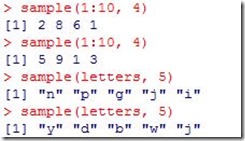
The sample function draws randomly from a specified set of (scalar) objects allowing you to sample from arbitrary distributions (sample space).

if you didn’t specified the number of values you want, sample will give you random permutation of the sequence.

as you noticed, by default sample will not repeat values, set parameter replace= TRUE to make it repeat .

Probability distribution functions

Probability distributions usually have four functions associated with them. The functions are prefixed with:

• r for random number generation
• d for density
• p for cumulative distribution
• q for quantile function

some useful distributions are:

Nickname	Distribution	For more information
norm	normal distribution	?Normal
pois	poisson distribution	?Possion
binom	binomial distribution	?Binomial
geom	geometric distribution	?Geometric
t	students t distribution	?TDist
f	F distribution	?FDist
chisq	Chi-Squared distribution	?Chisquare

function names are : prefix + distribution nickname. rnorm, rpois, rbinom,….. –> for random number generation, and so on.

In this note we introduced the basic functions for random number generation based on variable distribution type, arbitrary random sampling, and the associated probability distributions functions. Later will present each of them in detail.

Stay tuned for more R notes.

Introduction to R – Basic Debugging

In this post we will talk about native debugging support in R. Mostly, you start debugging when something goes wrong, which have many indications:

• message A generic notification/diagnostic message produced by the message function; execution of the function continues.
• warning An indication that something is wrong but not necessarily fatal; execution of the function continues; generated by the warning function; you got it after the function completion.
• error An indication that a fatal problem has occurred; execution stops; produced by the stop function.
• condition A generic concept for indicating that something unexpected can occur; programmers can create their own conditions.

The primary tools for debugging functions in R are:

traceback() prints out the function call stack after an error occurs; does nothing if there’s no error.

debug(f) flags a function for “debug” mode by setting a breakpoint at the beginning of the function f which allows you to step through execution of a function one line at a time. Use undebug() to turn off debug mode for that function. The debug mode turned off automatically when reloading your code using source().

When you execute your code and hit a breakpoint, you enter the debugger which called the browser in R. The command prompt will be something like Browse[2] instead of just >.

Then you can invoke various debugging operations operations:

• n or Enter to step through single line of code. If it is a line-level breakpoint, you have to hit n the first time, then Enter after that.
• c to skip to the end of the current context (a loop or a function).
• where to get a stack report
• Q to exit the debugger and return to the > command line.
• All normal R operations and functions are still available to you. So for instance to query the value of
  a variable, just type its name, as you would in ordinary interactive usage of R. If the variable’s name
  is one of the debug() commands, though, say c, you’ll need to do something like print(c) to print it
  out.

browser() suspends the execution of a function wherever it is called and puts the function in debug mode.

recover allows you to modify the error behavior so that you can browse the function call stack. It’s a global option that applies for the current global environment. You set it by calling options(error = recover) after that, any functions causes an error to occur you will get function call stack (like the one you got from traceback) with the option to jump into debugging any function that call stack.

trace() allows you to insert debugging code into a function at specific places. For example trace(f, t) would instruct R to call the function t() every time we enter the function f(). This helps if you want to put a breakpoint in the beginning of a specific function in your code file without opening the file, modifying the function, reloading the file using source(). You can just call trace(Your_Function, browser) . When you done with debugging this function you can call, untrace(Your_Function) to remove that debugging feature from your function.

These are interactive tools specifically designed to allow you to pick through a function. There’s also the more blunt technique of inserting print/cat statements in the function.

Stay tuned for more R notes.

Introduction to R – Control Structures

Like every other programing language, R have control structures that allow you control the flow of your code execution.

If, else for testing a condition. else section is optional.

if it’s all about assigning a value to a variable, you can do like this

for for executing a loop for a fixed number of times. It takes a variable and assign it successive values from a sequence or vector.

while for executing a loop while a condition is true. It begins by testing that condition, if it is true, the loop body will execute, if not, R will skip the loop.

repeat for executing an infinite loop; the only way to exit the loop is to call break

break for breaking the execution of a loop and continue from the next line of code after the loop (just like in the previous example)

next is used to skip an iteration of a loop

Writing multiple lines of code on the command-line interactive environment is hard. I have used the script editor to write the code in this post and then copied it to R console.

Loop functions

Loop functions is so similar to loops. It just more compact and easy to use on command line.

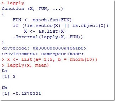
lapply loop over a list and evaluate a function on each element. If the first argument wasn’t a list, it will be coerced to a list (using as.list). lapply always returns a list. Any arguments passed to lapply beyonf the FUN parameter, will be assigned to the ellipsis and then passed as parameters to FUN. FUN can be an anonymous function.

sapply will try to simplify the result of lapply if possible. If the result is a list where every element is length 1, then it returns a vector. If the result is a list where every element is a vector of the same length (>1), it returns a matrix. If it can’t figure things out, it returns a list.

apply apply a function over the margins of an array. Often used to apply a function to rows and columns of a matrix. It takes as parameters the array; margin which indicates which dimension will be used as parameter to the function applied; and the function to be applied. In the example below, when passing 2 for the margin it means apply the function to columns, so we got a result of vector with length 10 containing the sum of each column. When we passed 1 for the margin, it means apply the function to rows, so we got a result of vector with length 20 containing the sum of each row.

for sums and means of matrix dimensions, we have some shortcuts:

• rowSums = apply(x, 1, sum)
• rowMeans = apply(x, 1, mean)
• colSums = apply(x, 2, sum)
• colMeans = apply(x, 2, mean)

tapply apply a function over subsets of a vector. It is equal to using split and lapply together. split take a vector or other objects and splits it into groups determined by a factor or list of factors.

mapply is a multivariate version of lapply. Each element will in 1:4 repeated by the corresponding number in 4:1.

In this post we introduced the basic control structured in R. Its almost the same in any c-like programming language.

Stay tuned for more R notes.

Introduction to R – Functions

Functions

Functions are just like what you remember from math class. Most functions are in the following form: f(argument1, argument2, ...) Where f is the name of the function, and argument1, argument2, . . . are the arguments
to the function. Here are a few examples of built-in functions:

Note in the last example that if you give the argument in the default order, you can omit the names. Some built-in functions have operator form like the following examples:

A function in R is just another object that is assigned to a symbol. You can define your own functions in R, assign them a name, and then call them just like the built-in functions. Writing your function code on the R Console is hard, so R provided a simple text editor for that. To write your code go to File >> New Script. This will open the R Editor, enter the following code


You could select the code, copy and paste it in R console. Now you can call the function to get its result (note that entering the function name and hitting enter retrieves the function code. This is a useful trick to view function code before using it).

Now lets go back to the editor and save the code in our working directory in MyCode.R (.R is the extension for R code files). To load the code in any R code file inside the console for use, use source() and pass the file name for it. Then you can use the code inside that file in the console. Each time you edit that code file, you have to call source() again to load the latest code.

Arguments

A function definition in R includes the arguments’ names (in the previous example we didn’t use any arguments).

Optionally, you can include default values for arguments. If you specify a default value for an argument, it will be considered optional (can be omitted from the function call). If you provided a value for an argument with default value, your value will override the default one. Non-optional parameters have to be provided in the function call.


If you want to specify a variable-length argument list, specify (…) in the arguments to the function. Everything other than the named arguments, will be stored in the ellipsis … .To can then convert the ellipsis to a list to work with it.

You can also refer directly to items within the ellipsis using the variables ..1 for the first item, ..2 for second and so on to ..9. Any argument that appear after the ellipsis in the function call, have to be named explicitly.
You can get the set of arguments accepted by a function, use the args function. NULL represents the function body.

You can pass named arguments any ware in the function call by their name. Unnamed arguments have to match the order that they are listed in the function definition. The following lm() function calls are equivalent :
lm(data = mydata, y ~ x, model = FALSE, 1:100)
lm(y ~ x, mydata, 1:100, model = FALSE)
Named argument are helpful if you have a long argument list which you remember it by arguments’ names, not the order.

Lazy Evaluation

Arguments to functions are evaluated lazily, so they are evaluated only as needed. The function below never uses the argument b, so calling f(2) will not produce an error because the 2 gets positionally matched to a (the only variable needed).

even if you will use a missing argument, R will not give an error until the first use of this missing argument. Everything before that will execute normally.

Return Values

You can use the return function to specify the value to be returned by the function. Also R will return the last evaluated expression as the result of the function if no return() is found.

Functions as Arguments

Many functions in R can take other functions as arguments. An example of these functions, the sapply function iterates through each element in a vector, applying another function to each element in the vector and returning the results.

Anonymous Functions

You create functions that do not have names. These are called anonymous functions. Anonymous functions are usually passed as arguments to other functions.

the R interpreter assigns the anonymous function functions(x) {x * 7} to the argument f of function apply.to.three then assigns 3 to the argument x of the anonymous function. So, it will ends up by evaluating 3 * 7 and returns the result.
anonymous functions can also be used with sapply()

it is possible also to define an anonymous function and apply it directly to an argument.

Scoping rules

How does R know which value to assign to which symbol ? How does R know what value to assign to the symbol lm ? Why doesn’t it give it the value of lm that is in the stats package ?

When R tries to bind a value to a symbol, it searches through a series of environments (sets of symbols, objects,…) to find the appropriate value. When you are working on the command line and need to retrieve the value of an R object, the search begins with the global environment you working in it and look for a symbol name matching the one requested. If not found, R starts searching the namespaces of each of the packages on the search list. You can get the search list using search() function. .GlobalEnv represents your current working environment on the R command line, and its always the first element of the search list. The base package is always the last one. The order on the list matters

If you loaded a package with library the namespace of that package will be in the 2nd position of the search list, and everything else will be shifted down the list.

You can also load package on the command line window by going to Packages >> Load package >> then select the desired package and click Ok.
You can configure which packages to be loaded automatically on startup to be available for you. To do that open C:\Program Files\R\<Your-R-Version>\etc\Rprofile.site using Notepad and append the following to the bottom of the file. You can append whatever package you want to the vestor c and it will be loaded for your on startup.
local({
old <- getOption("defaultPackages")
options(defaultPackages = c(old, "car", "RODBC", "foreign", "DAAG", "MASS",
"lattice ", "latticedl", "sciplot", "tree", "lme4"))
})
Lexical Scoping Rules (or Static Scoping Rules)  determines how a value is associated with a free variable in a function. The values of free variables are searched for in the environments in which the function was defined.
So what is a a free variable ? a free variable is not a formal argument (arguments declared in function signature) nor a local variable that is declared and assigned in the function body. In the following example, x and y are formal arguments. z is a free variable. f <- function(x, y) { x^2 + y / z }
So what is an environment ? an environment is a collection of (symbol, value) pairs. Every environment has a parent environment, and it is possible for an environment to have multiple children. A function + an environment = a closure or function closure.
So, searching for the value for a free variable starts in the environment in which the function was defined, if not found, the search continued to the parent environment. The search continues until we hit the top-level environment ( workspace or the namespace of the package). After that the search continues down the search list until we hit the empty environment. If not found, an error is thrown.
You can get the environment of a function using environment() (for functions coded on the command line, that will be the global environment). You can get the parent of an environment using parent.env() (for functions coded on command line, it will be send item in the search list).

Why does knowing lexical scoping rules matters ? Typically, a function is defined in the global environment, so that the values of free variables will be found in the user’s workspace (which is the right approach). However, in R you can define functions inside other functions, in this case the environment in which a function is defined is the body of another function.
In this post we talked about functions and using it weather from the console or from external files, functions as parameters, anonymous functions, and many other low level stuff.
Stay tuned for more R notes.

Introduction to R – Matrix Operations

Operations can be done on matrices in two fashions:

• Element-wise : where operations performed on corresponding elements in the matrices. Just use the desired operator.

• Matrix-wise: where operations are performed on the whole matrices in the way you used to do in math. Use the desired operator between a couple of % %

Stay tuned for more R notes.

Introduction to R – Removing missing values

A common task in preparing you data is to remove missing values(NAs). One way to do that is to retrieve a vector of the missing values in your data, and then filter them out from your structure.

If you want to filter out the missing values from more than one vector , you can use complete.cases() to get the indices that contains good data in both vectors.

Here good will contain TRUE only for indices that hold good data in both vectors; FALSE otherwise. complete.cases() works with data frames also. In that case it removes any row that contains NA in any column.The returned data frame will not contain any NAs.
Stay tuned for more R notes.